This week we check to see how much of our two choices of ordering the database, as entered and by year, are typical of random orderings. We test that by shuffling the order of the database 1,000 times, and then running the Heaps Law analysis one thousand times, one for each row or tune in the database. We then compare that outcome with the original two runs.
Here’s the plot of the Heaps’ Law beta that results from all thousand runs of the shuffled database:
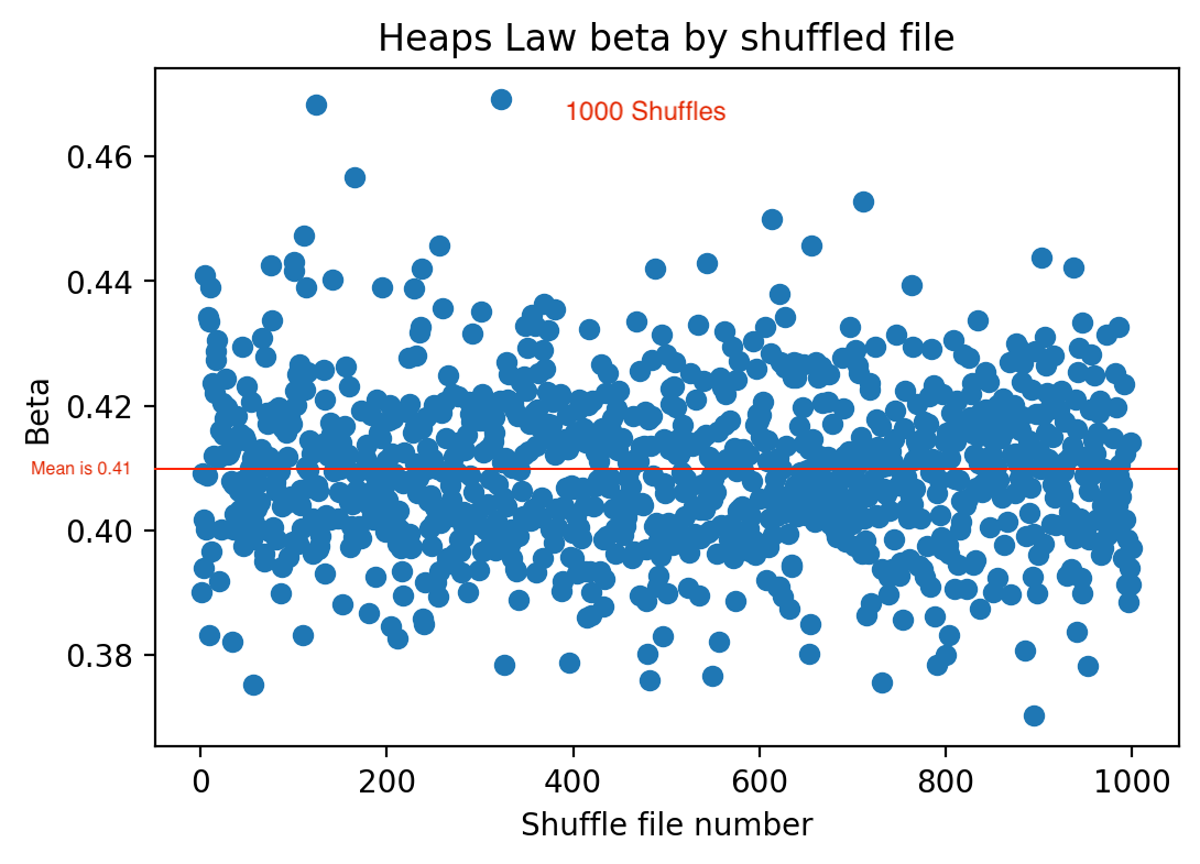
The vertical axis plots beta from the Heaps analysis and the horizontal axis plots each of the 1,000 shuffles of the database. Each blue dot represents the beta of one of those shuffles. The red horizontal line through the middle is the average beta value for all thousand runs. We see a pretty tight fit. The run with the highest beta value of a little over 0.46 one of the early shuffles, and the lowest was a little below 0.38 in one of the later shuffles. The standard deviation, which measures how tight the distribution is, had a value of 0.13. That means that we can have 95 percent confidence that the true beta value ranges from 0.39 to 0.43. For the record, the K value was 9.12, and the R-squared was 0.99, so the fit was quite good.
The stability of the beta values across all 1,000 runs is meaningful because it means the corpus has a highly consistent vocabulary-growth regime regardless of shuffle ordering. In other words, the melody vocabulary behaves as a mature statistical system. The extremely high R-squared value of 0.99 means the Heaps relationship is not merely approximate. The vocabulary growth follows a near-power-law extremely closely across nearly five million tokens. This is very similar to what is seen in natural language corpora.
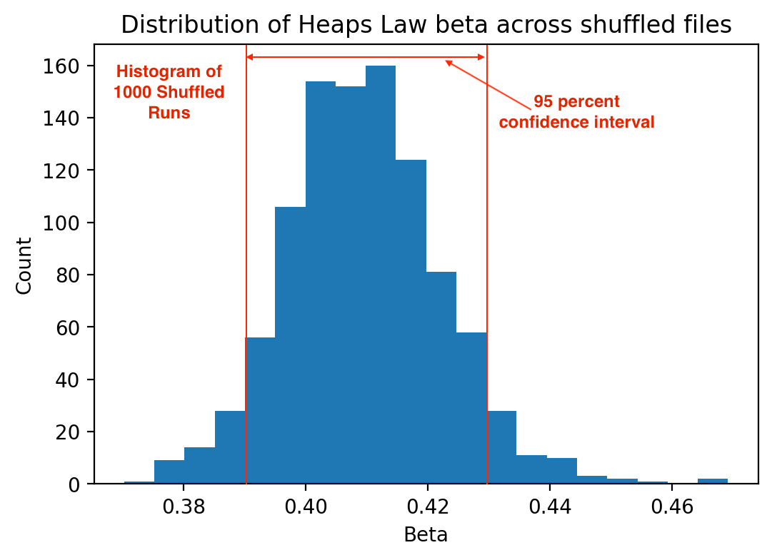
With 1,000 runs, we should get a nice histogram of the beta values, and indeed we do:
Heaps Curves
It’s instructive to treat the shuffled runs as a single Heaps Curve. Here’s what that looks like with the normal (not logarithmic) axes:
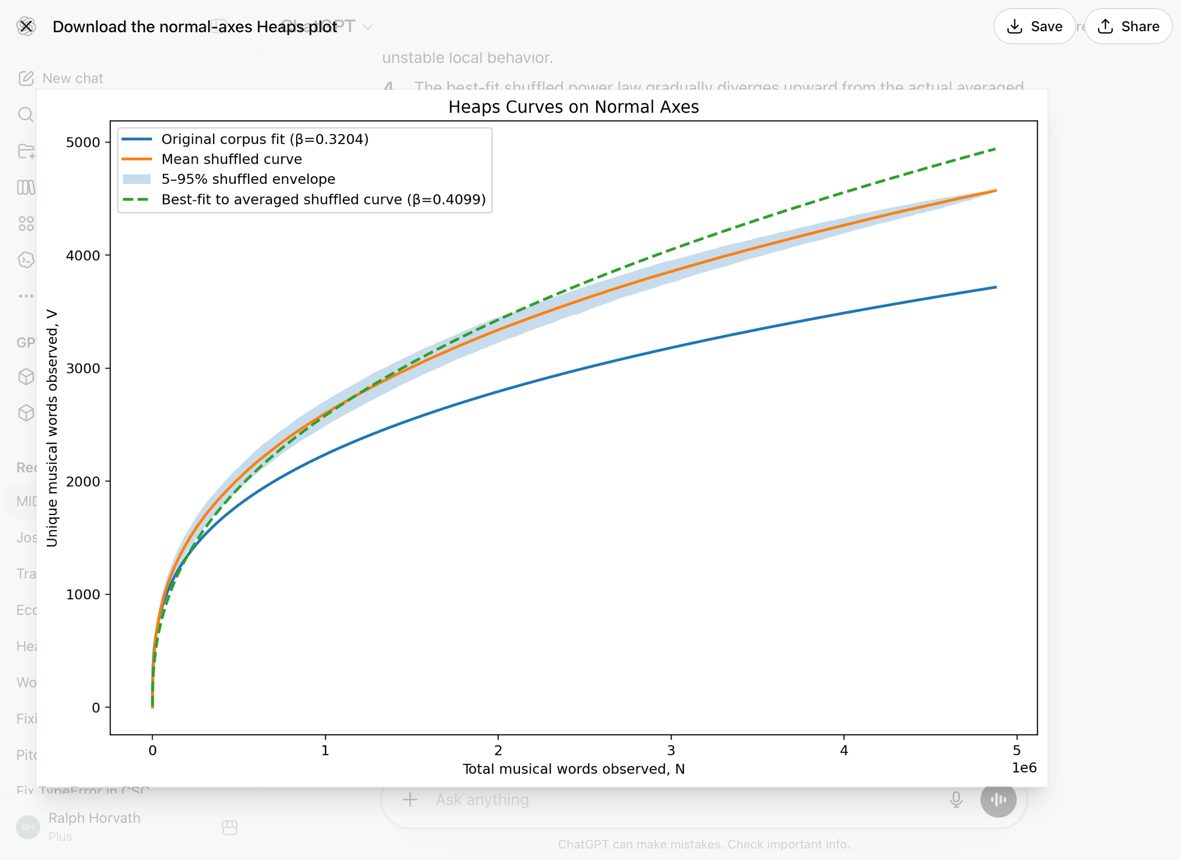
The normal-axis plot is great for visualizing actual vocabulary accumulation, and understanding the practical effect of corpus ordering. Plotted are the original corpus fit in blue (as entered, whose beta is 0.32), the shuffled fit in orange (along with the shaded light blue 5 to 95 percent deviations), and the fitted Heaps curve for the shuffled database using the mean beta of 0.41.
This normal-axis plot makes it clear that the original corpus ordering suppresses vocabulary growth substantially. The blue original-order curve falls far below the shuffled ensemble over most of the corpus. By the end of the corpus, the gap is on the order of several hundred token types. That is a very large effect statistically and musically.
The shuffled curves are extremely stable and the 5 – 95 percent envelope is remarkably narrow considering the 1,000 independent randomizations, nearly 5 million tokens, and thousands of vocabulary types. That means the vocabulary-growth dynamics are highly robust under random ordering.
The averaged shuffled curve is almost perfectly smooth, which strongly suggests the corpus has a stable large-scale lexical structure rather than unstable local behavior. The best-fit shuffled power law gradually diverges upward from the actual averaged shuffled curve late in the corpus, and that suggests mild sub-power-law saturation at the very largest scales. In other words, the finite vocabulary ceiling begins exerting pressure,
and true novelty growth slows slightly relative to the ideal infinite-vocabulary Heaps model. That is what one would expect from a constrained musical language.
Now let’s look at the log-log plot of the shuffled database:
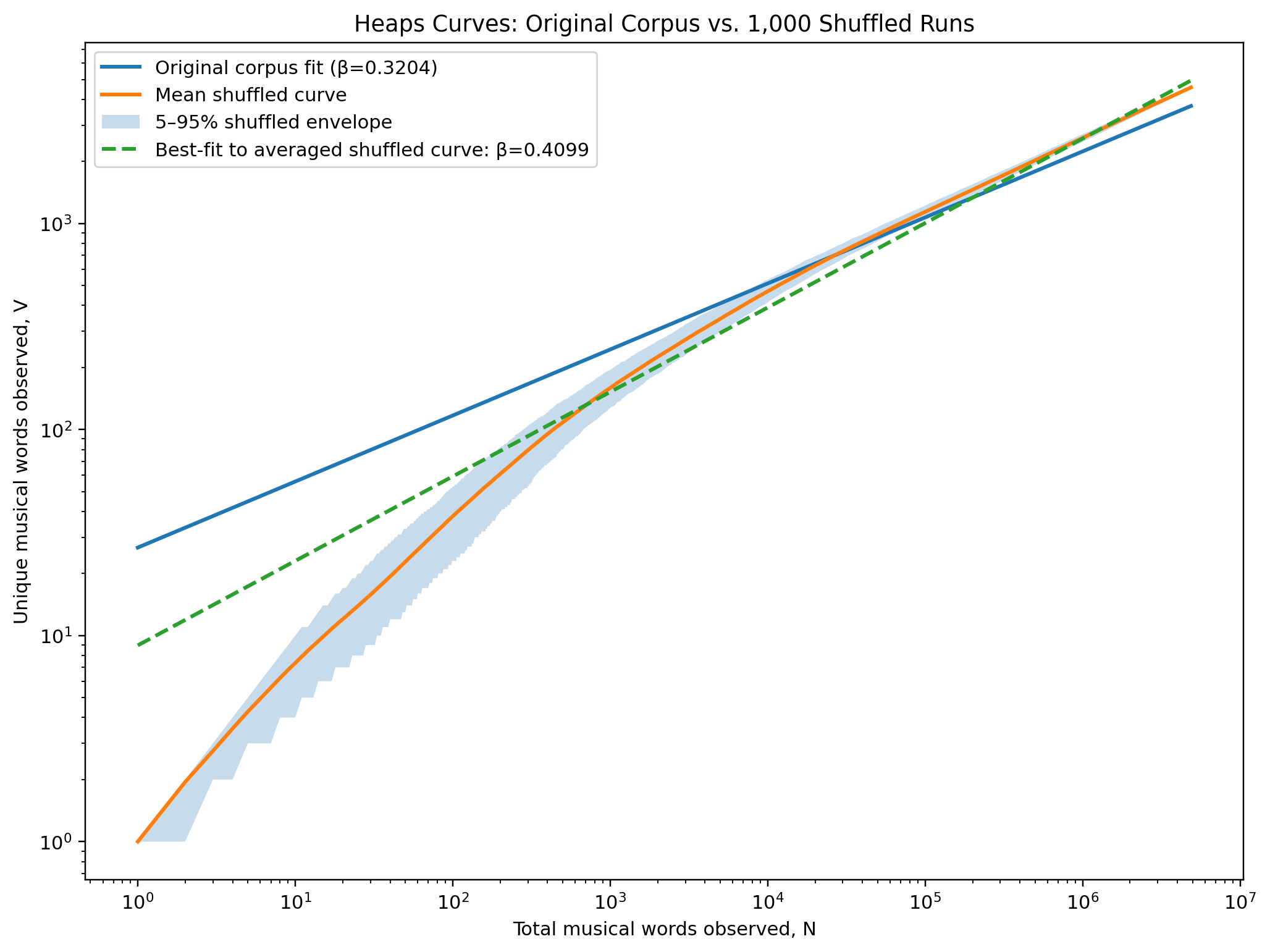
The combined log-log plot contains the same data as the previous plot, but on a logarithmic scale for both axes. The most striking feature is that the original ordered corpus diverges systematically from the shuffled ensemble. The shuffled mean grows more slowly at the very beginning, then overtakes the original curve and remains consistently above it through most of the corpus. That is what one would expect if our original entry order clustered stylistically related melodies together, which it does by intention.
The averaged shuffled curve itself fits a power law extremely closely with a β of 0.4099 and almost identical to the mean β from the 1,000 independent fits. That consistency strongly supports the claim that the vocabulary-growth behavior is an intrinsic statistical property of the corpus rather than an artifact of fitting noise.
Comparing All Three Betas
Let’s pull in the Heaps Curve results for the dataset when it was analyzed after being sorted by year. Here are all three betas:
β as-entered is 0.32 which is less than β chronological 0.38 which is less than β shuffled of 0.41
That hierarchy has a natural interpretation. The “as entered” database has the strongest local stylistic redundancy because we entered a chunk of the same kind of tune 100 times in a row. The “chronological” database has moderate historical continuity. And the “shuffled” database offers a basically random exposure to global vocabulary.
We tentatively conclude that most of the suppression in the original β = 0.32 came from our deliberate decision to enter by genre, but not all of it.
The year-ordered corpus still sits noticeably below the shuffled ensemble year-order β of 0.38 is well below (over two standard deviations) the shuffled mean β of 0.41, but those two are dramatically closer to each other than the as-entered β of 0.32. That last beta can’t even be seen on the above histogram because it is so far from the shuffled betas.
That implies two different kinds of clustering were operating. The first is strong artificial clustering from our chunky entry order, creating strong artificial clustering from database entry order and highly homogeneous local neighborhoods. That greatly delayed vocabulary discovery and suppressed β. Shuffling destroys this entirely, producing a β of 0.41
The second is residual historical and stylistic clustering in chronological order. The fact that year-order β rises to 0.38 but still remains below the shuffled mean suggests that musical vocabulary itself evolved historically in a correlated, gradual way.
Even when sorted only by year, nearby works still share stylistic vocabulary, eras have characteristic token distributions, innovations diffuse gradually rather than randomly, and local temporal neighborhoods remain statistically similar.
That is musically very plausible and consistent with our hypothesis that composers tend to stick with their familiar vocabulary until they can’t produce something that sounds new and fresh, only then inventing a new musical “word”.
Chronological ordering, therefore, still preserves genuine historical autocorrelation in melodic vocabulary, just not as much as when one deliberately enters tunes in genre.
That is probably why β remains below the shuffled baseline.
The fact that the 0.35 beta lies near the edge of the shuffled 95 percent interval is evidence that the effect is real rather than random. In other words, the chronological ordering is statistically distinguishable from random reorderings. We can reasonably say that ordering the corpus chronologically produces significantly slower vocabulary growth than random ordering, suggesting that melodic vocabulary evolves through temporally local stylistic continuity rather than through random sampling from a fixed global vocabulary.
That is a strong musicological claim, and while we can’t claim we’ve proved it yet, the Heaps Curve analysis provides some solid evidence in favor of it.
Equally interesting is that the difference between a beta of 0.32 (“as entered”) and 0.38 (chronological) essentially measures the extent to which our own editorial grouping amplified stylistic locality beyond what already exists historically.
We accidentally created a kind of “maximum clustering” experiment.
This post closes out our look at the Heaps Law as applied to notes (a pitch and its duration). The implications we can draw so far with respect to training an AI model is that embeddings stabilize quickly, and the vocabulary does not explode combinatorially the way natural language often does. We conclude that the note would be a reasonable choice for a “word” in a language-like Transformer AI training model. Compared to human language, our melody corpus appears language-like in statistical form but much more constrained, more repetitive (with the pitch-duration pairings), and more compressible.
Next week we turn to pitch differentials and duration ratios. Doing so treats two consecutive notes as a word, thereby expanding the vocabulary. Our guess, based on the analysis to date defining a “note” as a “word” is that the Heaps Curve analysis will continue to show robust language-like structures, both visually and statistically.