We now turn our attention to Heaps’ Law when our musical word is defined not as a single note, but as a note followed by the next note in a melody. This 2-note pairing will increase the vocabulary size, so we would expect results placing the Skiptune database a little closer to Heaps’ Curves as seen in human language than we did with single notes.
Our musical word is defined very precisely: A pitch differential followed by a duration ratio. The pitch differential is the pitch (MIDI value) of the second note in each pair less the pitch of the previous note. Likewise, the duration ratio is the duration of the second note divided by the duration of the first note. Here are a few examples of how notes on a staff are turned into a musical “word” using pitch differentials and duration ratios:
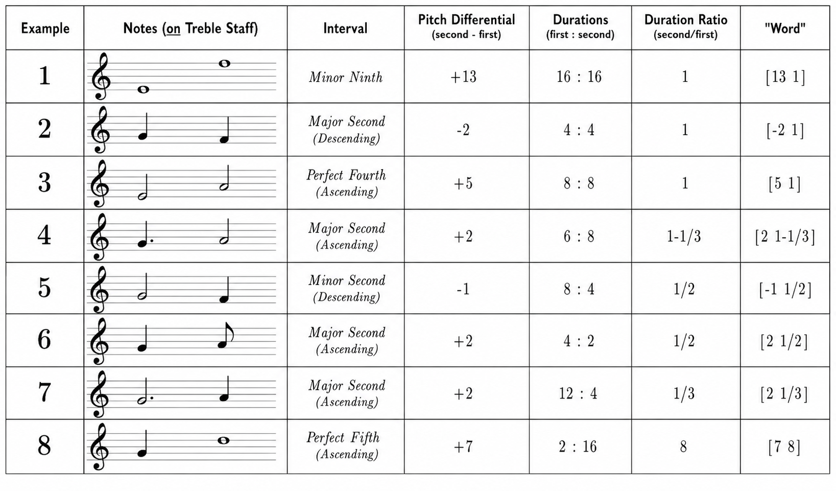
This chart shows how we go from two notes on a musical staff in treble clef to defining those two notes as a word for purposes of our Heaps’ Curve. Using the top row as an example, the staff shows an E at the bottom of the treble clef for the first note, which ascends to an F at the top of the treble clef. This is a Minor Ninth as shown in the next column for a total of 13 semitones in the column labeled “Pitch Differential”. Whole notes have a duration of 16 and each is a whole note as shown under Duration. Because 16 divided by 16 is 1, we have a Duration Ratio of 1. Finally, in the last column, we have our musical “word”, [13 1]. This token represents not just E to F a minor ninth above, but any pair of notes with the same duration a minor ninth apart ascending. For instance, an F quarter note to a G-flat quarter note a minor ninth away would also be represented by this token word.
Here’s the first tune of the database after being prepared for the Heaps analysis to put it in context for you. You wouldn’t know it from looking at it, but this is the tune to “Baa, Baa Black Sheep” in a form that can be analyzed:
[+0 1] [+7 1] [+0 1] [+2 1/2] [+0 1] [+0 1] [+0 1] [-2 4] [-2 1/2] [+0 1] [-1 1] [+0 1] [-2 1] [+0 1] [-2 2] [+0 1/2] [+0 1/2] [+0 1] [+7 2] [+0 1/2] [+0 1] [+2 2] [+0 1/2] [+0 1] [-2 3] [+0 1/3] [-2 2] [+0 1/2] [+0 1] [-1 1] [+0 1] [+0 1] [+0 1] [-2 2] [+0 1/2] [+0 1] [-2 4]
We’re ready to see how the Heaps’ Curve looks when we run the analysis on the database as entered using a word defined as a pitch differential and duration ratio tuple:
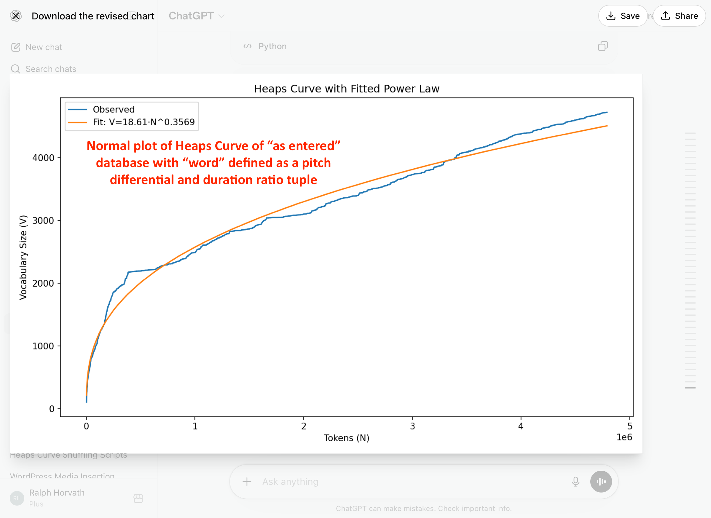
Our first reaction is that the observed blue line of the Skiptune data lies pretty close to the fitted Heaps Curve line most of the time. At first glance it doesn’t appear too different from the Heaps Curve when “word” was defined as just a note, not a pair of notes.
However, the numbers tell a different story. The beta value for the above curve is 0.36, higher than the 0.32 value for “word” defined as a single note. But compared to natural language, a beta of 0.36 is still relatively low, indicating substantial reuse of existing melodic intervals and rhythm patters.
We know the fit is quite good because the R-squared value is 0.977, rather strong. The power-law approximation remains an excellent description of vocabulary growth. The vocabulary size is also substantially increased: From 3,940 words when a word is a single note, the vocabulary rises to 4,720 when a word is a pair of notes. We knew it had to increase if only to accommodate notes moving to and from rests.
Let’s look at the log-log plot:
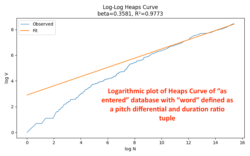
Each axis is plotted as the logarithm of the number of the number of tokens on the horizontal axis and the logarithm of the vocabulary size on the vertical axis. We see the database in blue working to catch up to the fitted orange curve, which means early melodies reused a relatively limited set of note-pairs, and that new tuple discovery accelerated later.
Around log 8 on the horizontal axis there is a notable jump. That steep section suggests a period where many new tuple types entered the database. When exactly will take further analysis, but it’s probably the baroque period.
The right-handed side is the most important part because from roughly log10 onward on the horizontal axis, the two curves are remarkably and notably close, telling us that melodies had entered a statistically stable regime.
As in the prior posts analyzing the rise of musical vocabulary using single notes, there is no sign whatsoever of saturation of musical language. That is, we keep seeing new note pairs emerging. If they were not, the blue line would begin bending downward and flattening toward the end. New tuples are still appearing, and the discovery rate is slowing, but the process has not yet approached a hard ceiling.
Next week we’ll look at the Heaps Curve using two-note tuples of the database sorted in order of composition or publication. If our experience with doing that using individual notes as a “word” is any indication, we’ll see a higher beta value that’s even closer to that of human language.