Because music is continuous rather than discrete, we do not find clean clusters of tunes. Instead, the boundaries between the clusters are completely occupied by borderline tunes–tunes that could easily be classified in one cluster or another.
While that finding was expected, we made another discovery that is somewhat troublesome: Tune length is strongly associated with cluster membership. Although the clustering algorithm did not use tune length as an explicit metric, the assignments show a very strong relationship with the number of sounded notes.
Note Count in Each Cluster
Consider this graph:
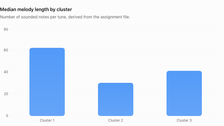
The column chart shows that Cluster 1 has tunes with the most notes on average, over 60 per tune. Cluster 2 has less than half that, and Cluster 3 is squarely between those two.
Cluster summaries hide detail, so let’s drill down with this table:
| Length of tune | Cluster 1 | Cluster 2 | Cluster 3 |
| 16 notes or fewer | 0.6% | 79.6% | 19.8% |
| 17–24 notes | 3.3% | 74.2% | 22.5% |
| 25–32 notes | 11.8% | 61.5% | 26.7% |
| 33–48 notes | 37.1% | 34.9% | 28.0% |
| 49–64 notes | 63.6% | 10.7% | 25.7% |
| 65–96 notes | 81.0% | 1.8% | 17.2% |
| 97–128 notes | 90.2% | 0.1% | 9.7% |
| Over 128 notes | 92–95% | ~0% | 5–8% |
This table drives home the point. Each row shows the distribution of tunes of that length across the three clusters, rather than the length distribution within an individual cluster as the graph did.
Nearly 80 percent of tunes containing 16 or fewer notes belong to Cluster 2, while more than 90 percent of melodies longer than 96 notes belong to Cluster 1. That raises the possibility that the algorithm has discovered three groups partly defined by length rather than three independent melodic styles, and that’s a problem.
Recall that several of our metrics normalize by note count, but that does not guarantee statistical independence from length. For example, the fraction of patterns occurring only once is naturally sensitive to the number of opportunities for repetition. A 20-note melody and a 100-note melody drawn from the same underlying musical process can have markedly different pattern statistics. Likewise, pitch range tends to increase as more notes are sampled, even if the underlying pitch distribution remains unchanged.
Feature or Bug?
That the clusters are strongly affected by tune length does not invalidate the cluster analysis. Rather, it identifies a potentially important confounding variable, tune length. For instance, Cluster 3 lies between the others in length, but exhibits a very pronounced repeated-pitch signature. That suggests the algorithm is finding structural variation beyond length alone.
The way to address this issue is to re-run the analysis while controlling for length.
More Clusters?
While our preprocessing choices are methodologically sensible, there may be other sensible choices as well we did not explore. Nonetheless, the analysis used 25 metrics grouped into conceptual families, with equal total squared-distance weight per family, and found reasonable clustters. That prevents a family containing many correlated metrics from dominating solely because it contributes more columns.
Our scaling was robust, 0.5th to 99.5th-percentile winsorization, a statistical technique used to limit the influence of extreme values (outliers) in a dataset, and ten initializations. The winning solution converged in 21 iterations without parsing warnings, a sign of a solid cluster analysis.
However, those are safeguards against numerical and weighting problems. They do not establish that three clusters are optimal. The reported two-dimensional visualization shown last week captures only part of the information. The variation explained by the first two visualization axes are 22.2 and 16.3 percent, respectively, for a total of just 38.5 percent. In other words, the remaining 61.5 percent lies in dimensions that the plot does not display.
This means that any visual overlap between clusters in the PCA picture does not necessarily mean that the groups are poorly separated in the full 25-metric space. Conversely, visually distinct concentrations in two dimensions do not establish robust separation.
Furthermore, our nearest-centroid and boundary data show that assignments have varying degrees of ambiguity. Some boundary tunes have almost identical distances to their nearest and second-nearest centroids, rendering the classification a bit arbitrary and random. The categories should thus be understood as approximate regions within a continuous musical feature space, not rigid natural classes.
Another qualification concerns missing values. The two rest-transition metrics have approximately 30,000 missing observations each. Our normalized, missing-value-aware distance calculation is a reasonable solution, but it means different tunes may be compared using different subsets of the 25 metrics. We would need to examine whether the missing data varies systematically by cluster.
Next Steps
The observation about note length and the three clusters is troubling enough to explore, so the next experiment is to control for tune length. Specifically, we will rerun the analysis on a common length range, such as 32 to 64 sounded notes, while keeping the same 25 metrics and preprocessing strategy. That would remove much of the dramatic length variation without requiring changes to the metrics.
We would then compare that result with the existing 3-cluster analysis. We can expect one of two outcomes: Either the same basic three profiles reappear, supplying stronger evidence that the cluster analysis has identified intrinsic melodic patterns, or our clusters disappear or reorganize. That would suggest that their apparent separation was strongly influenced by tune length.