Last week we found that Heaps’ Law applies well to the Skiptune corpus of melodies with a beta value of 0.36 using a note as a “word”. But as we observed, the order in which a computer reads in the database can affect the curve fit, so this week we check that out to see if our order of entry was representative of music as a language.
For the record, our entry of the melodies started with nursery tunes because they were simple and we could test whether the MIDI representation using Lilypond notation would work. From there we simply started collecting any source that provided the meta data we needed (year of composition or at least publication, composer name if known, labels, etc.). Two worthy of mention are Flute Tunes and Hymnary. The former has a lot of music written specifically for flute, but also has a wide variety of tunes written over time stretching back centuries. The latter contains tens of thousands of Christian hymns, also well curated. In both cases, the music was all in the pubic domain.
As we were entering these melodies, we started purchasing tune books and entering their melodies. Over time, we developed an approach whereby we entered 100 tunes from the 1700s or before, the 1800s, and the 1900s, wrapping around to the renaissance or baroque eras to repeat the process every 300 tunes. So while there is a kind of system to the entry, and it was definitely not random, there was no intentional order except to make sure we had good representation across the centuries. But we didn’t know, until now, how that order might affect application of analyses like Heaps’ Law.
The Heaps’ Law beta value of 0.36 we found last week was computed based on the system of entry described above. To find out if the order matters in the analysis, we first reorder the melodies so they are in order of composition (or, when that’s unknown, publication). When we do that, we get a beta value of 0.52, which is quite striking because it’s much higher than the 0.36 value calculated using the entry order of the database. Here’s what the Heaps analysis looks like visually in the regular plot (no logarithms):
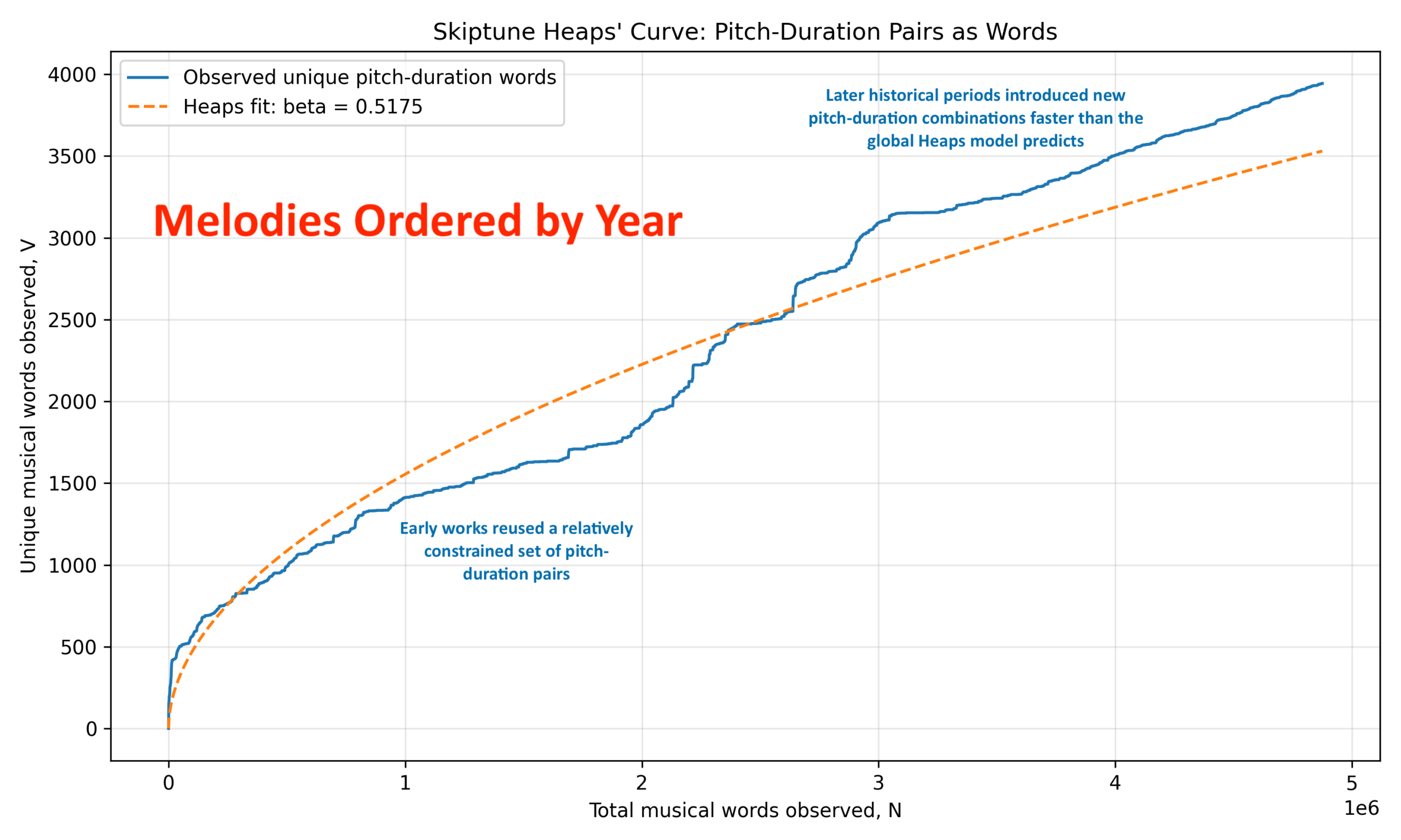
Because the corpus is ordered chronologically, the curve is no longer merely how vocabulary (different notes) grows with sample size, but also how musical vocabulary evolved historically. The plot appears to show roughly three phases.
- Phase 1 — Early Saturation. The left side of the blue plot rises quickly initially, then begins flattening relative to the fitted orange curve. That suggests many early musical works reused a relatively constrained set of pitch-duration pairs, which makes sense as our major and minor scales, unadorned by accidentals (sharps and flats) were being developed, along with rhythmically regular combinations. This is exactly what one would expect from early tonal music, folk material, and dance-derived repertories. In this phase total vocabulary rises rapidly, but genuinely new pitch-duration combinations appear more slowly. That is, vocabulary reuse dominates innovation.
- Phase 2 — Accelerated Innovation. Around the middle of the plot, the observed curve catches up to, fits quite well for a brief bit, and then exceeds the fitted Heaps curve in orange. This is perhaps the most important feature in the plot because it suggests that later historical periods introduced new pitch-duration combination faster than the global Heaps model predicts. That is potentially musicologically meaningful. Reasons might be chromaticism expansion (use of notes not in the diatonic scales mentioned in Phase 1), rhythmic diversification, Romantic-era phrase complexity, ragtime and jazz syncopation, and rock vocabulary. Our hypothesis that composers gradually exhaust common combinations is at least compatible with this observed curve. The especially sharp upward jumps between 2 and 3 million words represent bursts of vocabulary innovation and future work would see what eras (romantic? jazz? rock?) this corresponds to. The plot does not tell us when this occurs, and that exercise is left for a future project.
- Phase 3 — Persistent Growth Without Saturation. The far-right tail continues climbing strongly. Even after nearly 5 million tokens (notes), the vocabulary still grows noticeably. That means the pitch-duration vocabulary is not close to saturation, strong evidence against the idea that melodies only use a tiny closed vocabulary.
Now let’s turn to the log-log plot:
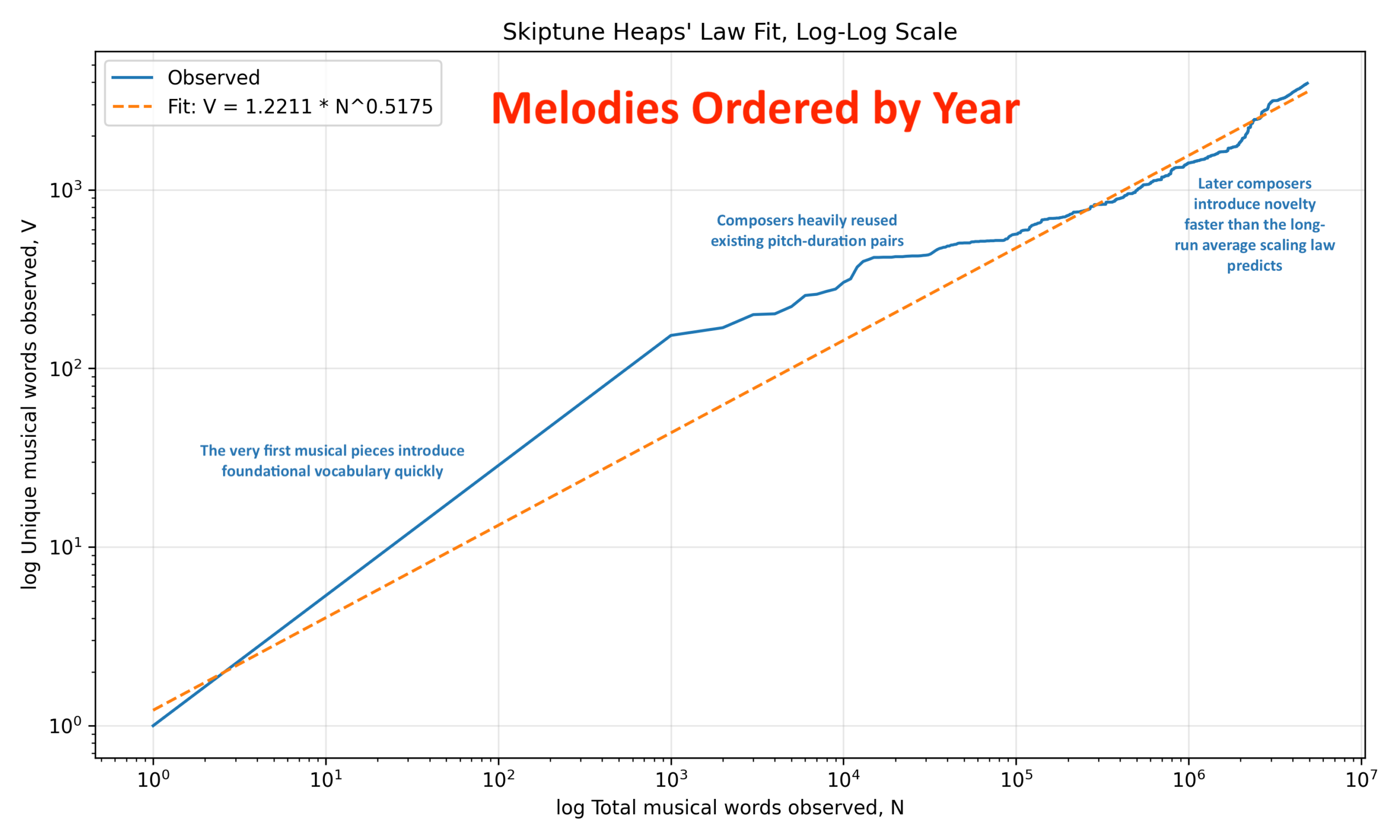
Classic Heaps’ law usually assumes random or natural sequential sampling. But here the corpus has been deliberately sorted by year. That means the Heaps’ curve conflates statistical vocabulary growth with historical musical evolution. We are effectively measuring “diachronic lexical innovation in melody space,” which just means how the musical vocabulary has evolved historically. That is in addition to what we learn from the ordinary Heaps’ curve. In other words, we are tracking the historical expansion of the melodic lexicon through time.
The advantage of the log-log plot over the first, linear plot is that it straightens out the fitted Heaps curve to a straight line, allowing us to easily see how the Skiptune corpus deviates from how note-duration pairs might have developed if it followed Heaps’ Law perfectly.
The log-log curve tells you something fundamentally different from the ordinary (“linear”) Heaps curve. The ordinary curve emphasizes: absolute vocabulary growth over time, whereas the log-log curve emphasizes scaling behavior and proportional growth. That distinction is useful because on the ordinary plot you mainly notice flattening, bursts, accelerations, and historical era changes. On the log-log plot you are looking for straightness, slope, curvature, and local deviations from power-law behavior.
The single biggest conclusion from the log-log plot is that the Skiptune pitch-duration vocabulary behaves approximately like a power law over several orders of magnitude, which is nontrivial. The corpus spans from 1 token to nearly 5 million tokens, yet the relationship remains broadly close to linear on log-log axes. That is exactly what Heaps’ law predicts.
The fitted slope β equals 0.52 means vocabulary growth is sublinear but persistent. That is the key theoretical statement because sublinear means new words become rarer as the corpus grows, and it’s persistent because the novelty of new vocabulary hasn’t yet disappeared entirely.
In practical musical terms, early on, almost every new token introduces a new word. Later, most tokens are repetitions, but genuinely new pitch-duration combinations continue appearing.
Now compare that to the ordinary plot at the top of this page. The ordinary plot made it look as though later music suddenly exploded with novelty. The log-log plot moderates that interpretation somewhat because on log-log axes proportional growth matters, not absolute growth, and the log-log curve remains surprisingly close to linear overall. In other words, despite historical changes, the underlying scaling structure remained fairly stable across millions of observations. So the ordinary plot emphasizes historical bursts, while the log-log plot emphasizes long-range statistical regularity.
Now let’s discuss the deviations The log-log curve is not perfectly straight. You can see early upward deviation, middle flattening, and later upward re-acceleration. Those departures from straightness are probably the most musically interesting feature.
If the curve were perfectly straight, the same vocabulary-generation process would dominate all eras equally. The bends in the curve suggest that the underlying generative process for new vocabulary changed historically.
Specifically, on the left in the early region, the observed (blue) curve initially rises above the fit, which means very early corpus growth produces vocabulary rapidly. That makes sense because the very first pieces introduce foundational vocabulary quickly.
Then the curve flattens relative to the orange fitted curve, meaning that composers started to heavily reuse existing pitch-duration vocabulary. This is a period of stabilization and “best practice” among composers as they learned from each other.
Toward the upper right, the curve rises again when later composers introduce novelty faster than the long-run average scaling law predicts (the orange line). The log-log curve also tells us something about saturation, which is that the curve does not strongly bend downward at the far right. That means vocabulary saturation is not occurring yet. If the musical vocabulary were approaching exhaustion, the log-log curve would curl sharply downward.
Another important observation is that a β of 0.52 is fairly high, which implies that the definition of a “word” here (pitch-duration) is relatively productive. If β had been, say, in the 0.1 to 0.2 range, it would have implied an extremely constrained vocabulary.
That completes the analysis of the Heaps’ Curve as applied to an ordered (by year) database. At this point we have quite different estimates of beta, 0.36 for the database as entered, and 0.52 for the database sorted by year. The first estimate suggests that a note “word” is a bit like human language words, but not too much, whereas the second estimate suggests that the note is very much like a human language.
To learn which of these is more correct, we need to see how sensitive our conclusions are to the order of the data base. Suppose a shuffled Skiptune corpus produces a smooth Heaps curve, but a chronological corpus produces systematic acceleration. Then we would have evidence that musical vocabulary itself historically expanded over centuries, suggesting that melody is not merely recombination inside a fixed vocabulary, but rather an expanding symbolic system with measurable historical innovation dynamics. That is a much stronger and more ambitious claim than ordinary Heaps’ law alone.
That’s next week.