This week we perform our last analysis of Heaps Law using 2-note words, and we do so by shuffling the database 1,000 times and performing a Heaps Law analysis on each one, calculating the statistical properties of that shuffled deck, and compare it to our year-ordered analysis. The results are highly informing.
We start with the shuffled run itself. Taken by themselves, the 1,000 runs tell us about the vocabulary-growth behavior we would expect if the same 83,400 tunes were presented in random order. The answer is that we have remarkable stability in vocabulary growth. Let’s take a look at the plot:
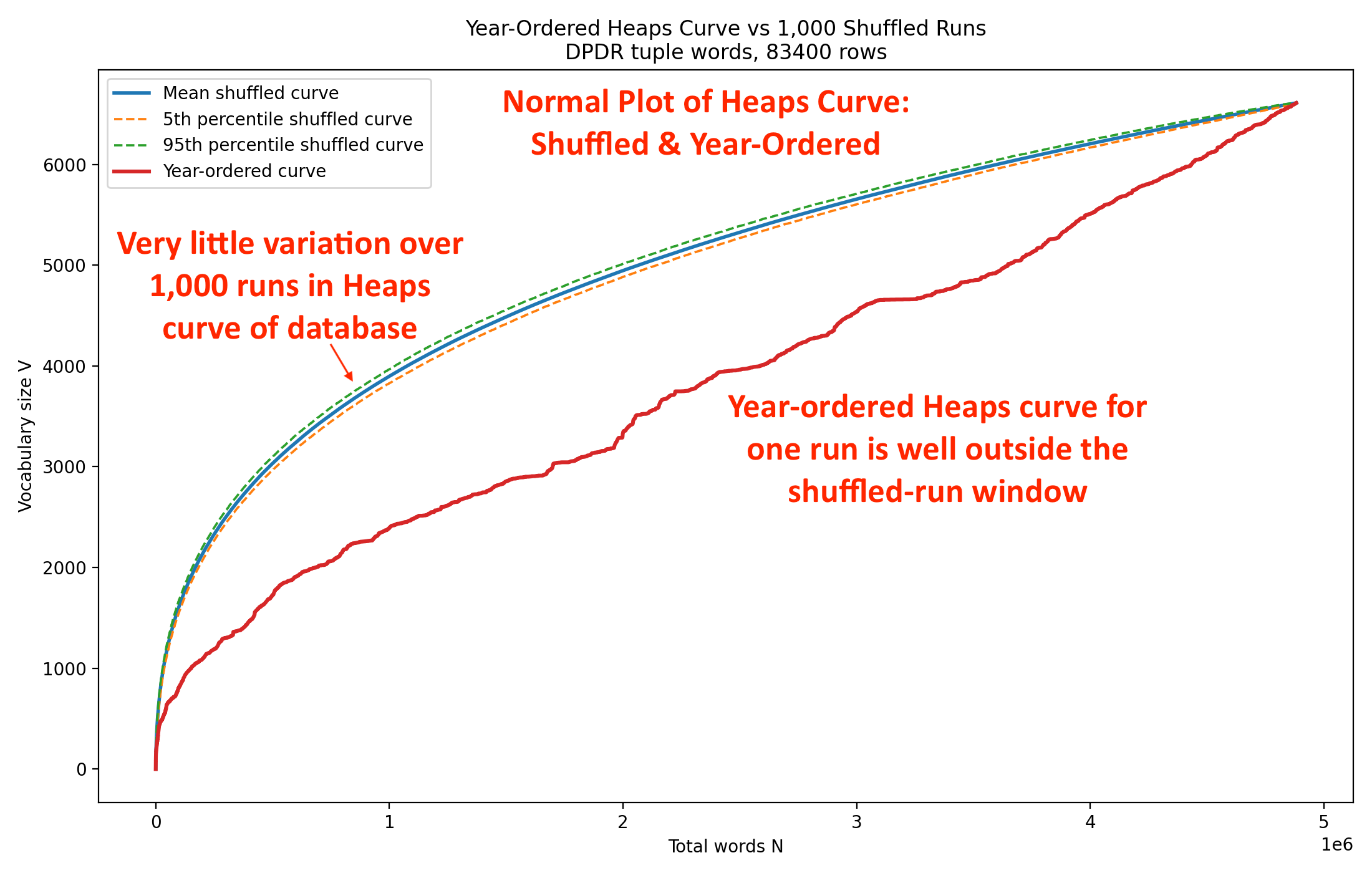
The envelope between the 5th and 95th percentile curves is quite narrow in the above plot. That envelope bounds virtually all the runs in a very small window width. You can see that the dotted boundary. lines are very tightly spaced from the blue average Heaps curve from the 1,000 runs.
The extremely tight range means that the shuffled result is highly reproducible, that the exact random shuffle doesn’t matter much and that the corpus has a well-defined baseline Heaps behavior.
We can think of the shuffled runs as establishing the “null model” from which we can compare runs that have some order to them. If tune order carried no information, the year-ordered curve (red line) should wander around inside that envelope. It does not. In fact, it stays pretty much entirely below the 95 percent confidence
That the red curve sits dramatically below the shuffled envelope for most of the corpus means that new vocabulary arrives much more slowly when the tunes are presented chronologically. In other words, earlier tunes are reusing vocabulary that later tunes will also use.
The year ordering is creating a strong vocabulary continuity effect. When you randomize the tunes, the corpus “discovers” vocabulary earlier. When you keep the historical ordering, vocabulary is revealed gradually over time. That’s exactly what you would expect if musical vocabulary evolves historically.
That vocabulary discovery is slower than the rate we’d expect from random vocabulary discovery is an important insight. Suppose musical vocabulary were not dependent on time. Then a year 1500 tune and a 1950 tune would essentially all draw from the same vocabulary. Shuffling would not matter much, and that fact that it matters tremendously means musical vocabulary is time-dependent. The chronological sequence delays the appearance of many tokens, and that is why the red curve remains below the shuffled curves.
Now let’s take a look at the logarithmic plot of the same data.
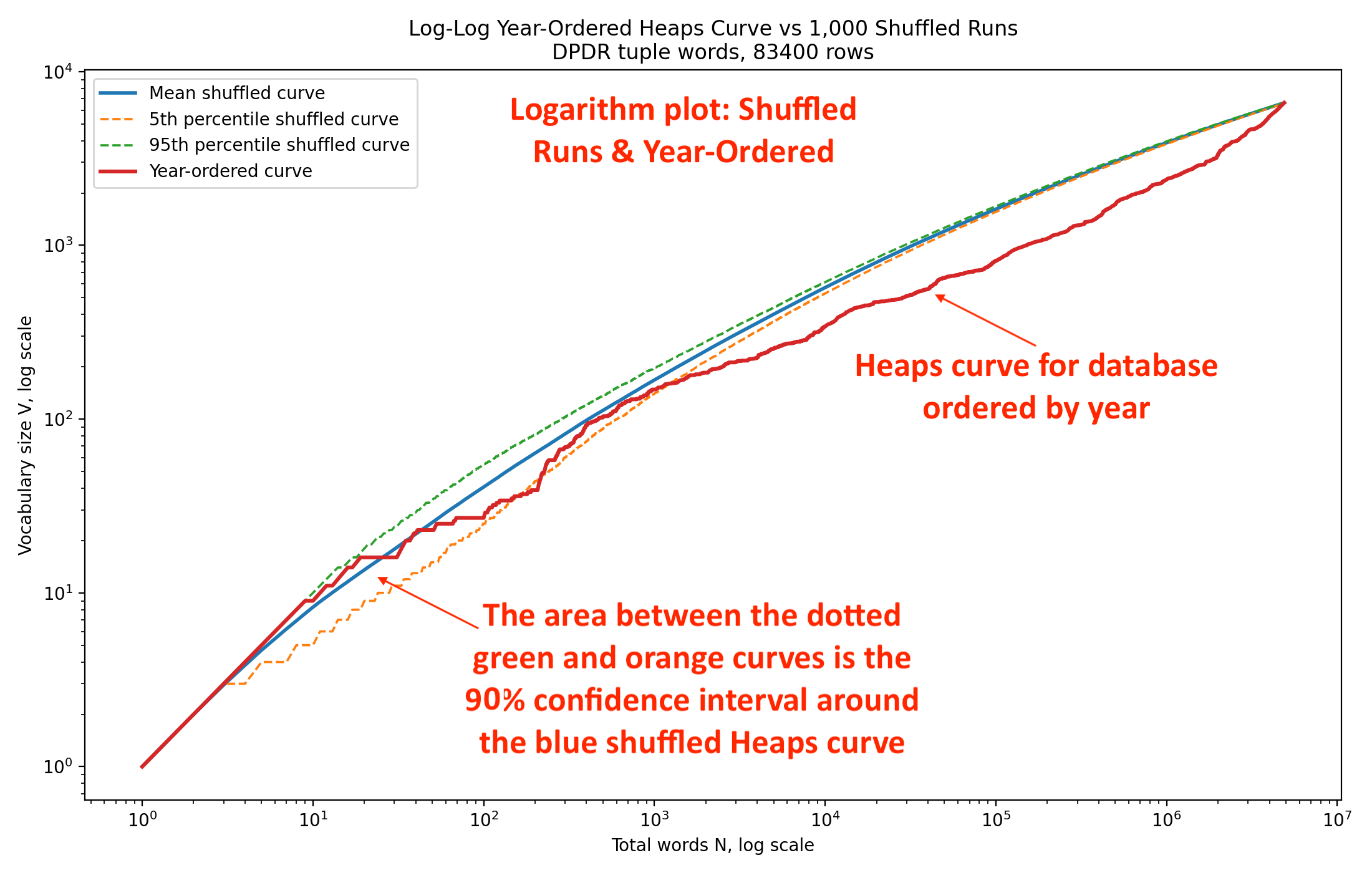
Taking the logarithm of each axis has the effect of condensing the earlier years and expanding our visualization of the later years. Notice that: the shuffled curves are close to straight, and that the year-ordered curve has long departures below the shuffled curve, indicating that the difference is not merely a startup effect. The effect persists across multiple orders of magnitude starting around when the musical vocabulary was only around 1,000 words. The separation is visible around across the rest of the corpus. From that, we know it is not caused by a handful of unusual tunes.
We interpret this analysis as suggesting that the Skiptune melodic vocabulary exhibits strong historical stratification. When melodies are presented in chronological order, new differential-duration (two-note word) vocabulary accumulates substantially more slowly than expected under random ordering. The effect is persistent across the full corpus and places the chronological curve below the 5th percentile of 1,000 random shuffles at approximately 87 percent of sampled points. This suggests that musical vocabulary evolves progressively through time rather than being uniformly distributed across historical periods.
The ramifications for later AI training are clear: We will need to incorporate the year each melody is associated with into any training model, as the statistical deviation from the highly stable shuffled curve is too large to ignore. The year each melody was composed or published carries a lot of information about existing vocabulary that we can’t afford to ignore if we expect the AI to recognize melodic differences based on different vocabularies.
Next week we wrap up our analysis of Heaps Curves with respect to the Skiptune musical corpus. We’ll summarize our findings and come to a conclusion about how to approach AI training when that time comes.